Fundamental relationship of the traffic flow交通流流密速关系阐述
Resource: Northwestern University, Yu(Marco) Nie, CIV-ENG 376 Lecture Notes
Notations 符号
| Symbols | Meaning |
|---|---|
| $q$ | Flow rate(pcu/h, vph) 流量 (How much the traffic flows) |
| $k$ | Density(pcu/km, vpm) 密度 (How crowd the road is) |
| $u$ | Space mean speed(km/h, mph) 空间平均速度 (how fast the traffic moves) |
| $\bar{v}$ | Time mean speed(km/h, mph) 时间平均速度 |
| $T$ | A period of time(h, min, s) 时间 |
| $N$ | Numbers of vehicles 车辆数量 |
| $x$ | Location 位置 |
| $t$ | A moment 时刻 |
| $h$ | Headway(s) 车头时距 |
| $s$ | Spacing (m, ft) 车头间距 |
| $i$ | index of vehicle 车辆编号 |
General Relationship 流密速通用关系
| Formulation | |
|---|---|
| basic relationship | $q=ku$ |
| General definition | $q=\frac{\text{Total travel distance}}{\text{Shaded area}}$ |
| $k=\frac{\text{Total travel time}}{\text{Shaded area}}$ | |
| $u=\frac{\text{Total travel distance}}{\text{Total travel time}}$ | |
| time mean speed is a flow-weighted speed | $\bar{v}=\sum_{i}\frac{q_i}{q}v_i$, $q=\sum_{i}q_i$ |
| space mean speed is a density-weighted speed | $u=\sum_{i}\frac{k_i}{k}v_i$, $k=\sum_{i}k_i$ |
| numerical relationship | $u\leq \bar{v}$ |
Two different observation methods for speed 观测速度的两类方法
There are two kinds of speed in traffic: the time mean speed and the space mean speed which have different definition. There are two ways to collect the speed and each method can collect both speed. The two methods have the following differences.
| Method 1 | Method 2 | |
|---|---|---|
| Observation method | Stand at roadside with a watch | Took photos on a helicopter |
| Single-x at $x_1$ | Single-t at $t_1$ | |
| info | $i$th vehicle arrival time $\tau_i$ headway $h=\tau_{i+1}-\tau_i$ * total vehicle passing $N$ within $T$ time | $i$th vehicle location $x_i$ spacing $s_i=x_{i-1}-x_i$ * total vehicles within $L$ |
| Cumulative count curve | $N - t$ diagram | $x- N$ diagram |
| Micro-macro relationship | $q$ with $\bar{h}$ | $k$ with $\bar{s}$ |
| $q=\frac{N}{T}=\frac{N}{\sum_{i}h_i}=\frac{1}{\sum_{i}h_i/N}=\frac{1}{\bar{h}}$ | $k=\frac{N}{L}=\frac{N}{\sum_{i}s_i}=\frac{1}{\sum_{i}s_i/N}=\frac{1}{\bar{s}}$ | |
| double-x | double-t | |
| supplement info | * $i$th travel time between $x_1, x_2$, which induce the travel speed $v_i=dx/dt_i=(x_2-x_1)/(\tau_i^\prime-\tau_i)$ | * Distance traveled y $i$th vehicle between $t_1$, $t_2$, which induce the travel speed $v_i=dx_i/dt=(x_i^\prime-x_i)/(t_2-t_1)$ |
| Time mean speed | $\bar{v}=\frac{1}{N}\sum_{i}v_i$ | $\bar{v}=\frac{\sum_{i}v_i^2}{\sum_{i}v_i}$ |
| Space mean speed | $u=\frac{N}{\sum_{i}1/v_i}$ | $u=\frac{1}{N}\sum_{i}v_i$ |
| Cumulative count curve meaning | horizontal: travel time of a particular vehicle between $x_1$ and $x_2$ | horizontal: # vehicles passing a location between $t_1$ and $t_2$ |
| vertical: at a time # vehicles between $x_1$ and $x_2$ | vertical: travel distance of a particular vehicle between $t_1$ and $t_2$ | |
Proof of the numerical relationship $u\leq \bar{v}$:
- In double-x method, From the Cauchy-Schwarz inequality, we have: $||\langle x,y\rangle||^2\leq \langle x,x\rangle\cdot\langle y,y\rangle$;
By setting $x=[\sqrt{v_1},\cdots, \sqrt{v_n}]^\intercal$ and $y=[1/\sqrt{v_1},\cdots, 1/\sqrt{v_n}]^\intercal$, we get $N^2\leq \sum_i v_i\cdot \sum_i \frac{1}{v_i}$, and then $\frac{N}{\sum_i \frac{1}{v_i}}\leq \frac{\sum_i v_i}{N} $ which indicates $u\leq \bar{v}$.
- In double-t method, similarly by setting $x=[v_1,\cdots, v_n]^\intercal$, $y=[1,\cdots, 1]^\intercal$, we get $(\sum_i v_i)^2\leq N(\sum_i v_i^2)$, and then $\frac{\sum_i v_i}{N}\leq \frac{\sum_i v_i^2}{\sum_i v_i}$, which indicates $u\leq \bar{v}$.
The derivation of the time mean speed and space mean speed in each method:
In double-x method: assuming $q_i=1$ because we view each vehicle as a flow stream of its own
- Time mean speed: $\bar{v}=\sum_{i}\frac{q_i}{q}v_i=\frac{1}{N}\sum_{i}v_i$
- Space mean speed: $u=\sum_{i}\frac{k_i}{\sum_{i}k_i}v_i=\sum_{i}\frac{q_i/v_i}{\sum_{i}q_i/v_i}v_i=\sum_{i}\frac{1/v_i}{\sum_{i}1/v_i}v_i=\frac{N}{\sum_{i}1/v_i}$, further we could have $u=\frac{N}{\sum_{i}1/v_i}=\frac{NL}{L\sum_{i}1/v_i}=\frac{NL}{\sum_{i}t_i}=\frac{L}{\frac{1}{N}\sum_{i}t_i}$
In double-t method: assuming $k_i=1$ because we view each vehicle as a flow stream of its own
- Time mean speed: $\bar{v}=\sum_{i}\frac{q_i}{\sum_i q_i}v_i=\sum_{i}\frac{k_iv_i}{\sum_i k_iv_i}v_i=\sum_i\frac{v_i}{\sum_{i}v_i}v_i=\frac{\sum_{i}v_i^2}{\sum_{i}v_i}$
- Space mean speed: $u=\sum_{i}\frac{k_i}{k}v_i=\sum_i\frac{1/L}{N/L}v_i=\frac{1}{N}\sum_{i}v_i$
How to get the general definition
Imagine a shaded area on the x-t diagram:
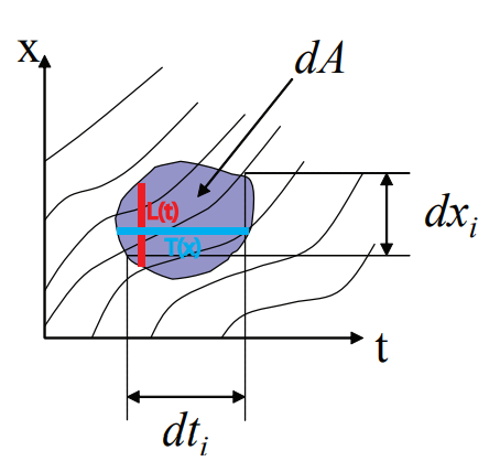
How to apply General definition into two observation method
Note that the area is shaded area in x-t diagram
- In double-x method:
- $\text{total travel distance}=N\times dx$, $\text{total travel time}=\sum_i dt_i$, $\text{The area}=dx\times T$
- $q=\frac{Ndx}{Tdx}=\frac{N}{T}$
- $k=\frac{\sum_i dt_i}{Tdx}$
- $u=\frac{Ndx}{\sum_i dt_i}=\frac{N}{\sum_i dt_i/dx}=\frac{N}{\sum_i 1/v_i}$
- In double-t method:
- $\text{total travel distance}=\sum_i dx_i$, $\text{total travel time}=N\times dt$, $\text{The area}=dt\times L$
- $q=\frac{\sum_i dx_i}{Ldt}$
- $k=\frac{N\times dt}{Ldt}=\frac{N}{L}$
- $u=\frac{\sum_i dx_i}{N\times dt}=\frac{1}{N}{\sum_i \frac{dx_i}{dt}}=\frac{1}{N}{\sum_i v_i}$
Greenshield’s model 交通流基本图关系之格林希尔治模型
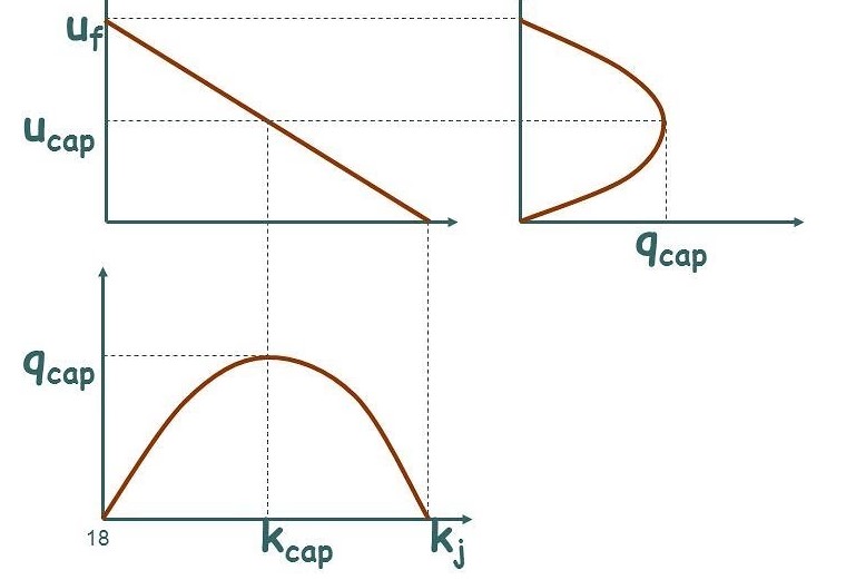
The Greenshield’s model is a
The critical properties:
$k_{cap}=\frac{k_j}{2}$
$q_{cap}=\frac{u_fk_j}{4}$
$u_{cap}=\frac{u_f}{2}$
Inductive loop detector traffic measurement 线圈检测器数据估计交通流状态
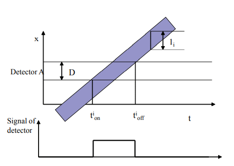
- $v_i=\frac{li+D}{dt_i}$, where $l_i $is the vehicle length and $D$ is loop detector width.
- $q=N/T$, where $T=30\text{ sec or } 5\text{ min}$.
- $u=\frac{\text{Total travel distance}}{\text{Total travel time}}=\frac{\sum_i(l_i+D)}{\sum_i dt_i}$
Occupancy $\rho$ is defined as the percentage of time when it is occupied. It is used to denoted density:
- $\rho=\frac{\sum_i dt_i}{T}\times 100=\frac{q\sum_i dt_i}{N}\times 100=\frac{q}{N}\frac{\sum_i (l_i+D)}{u}\times 100=\frac{k\sum_i (l_i+D)}{N}\times 100=k(D+\bar{l})\times 100\equiv kg_D$